User guide
Pivot reports

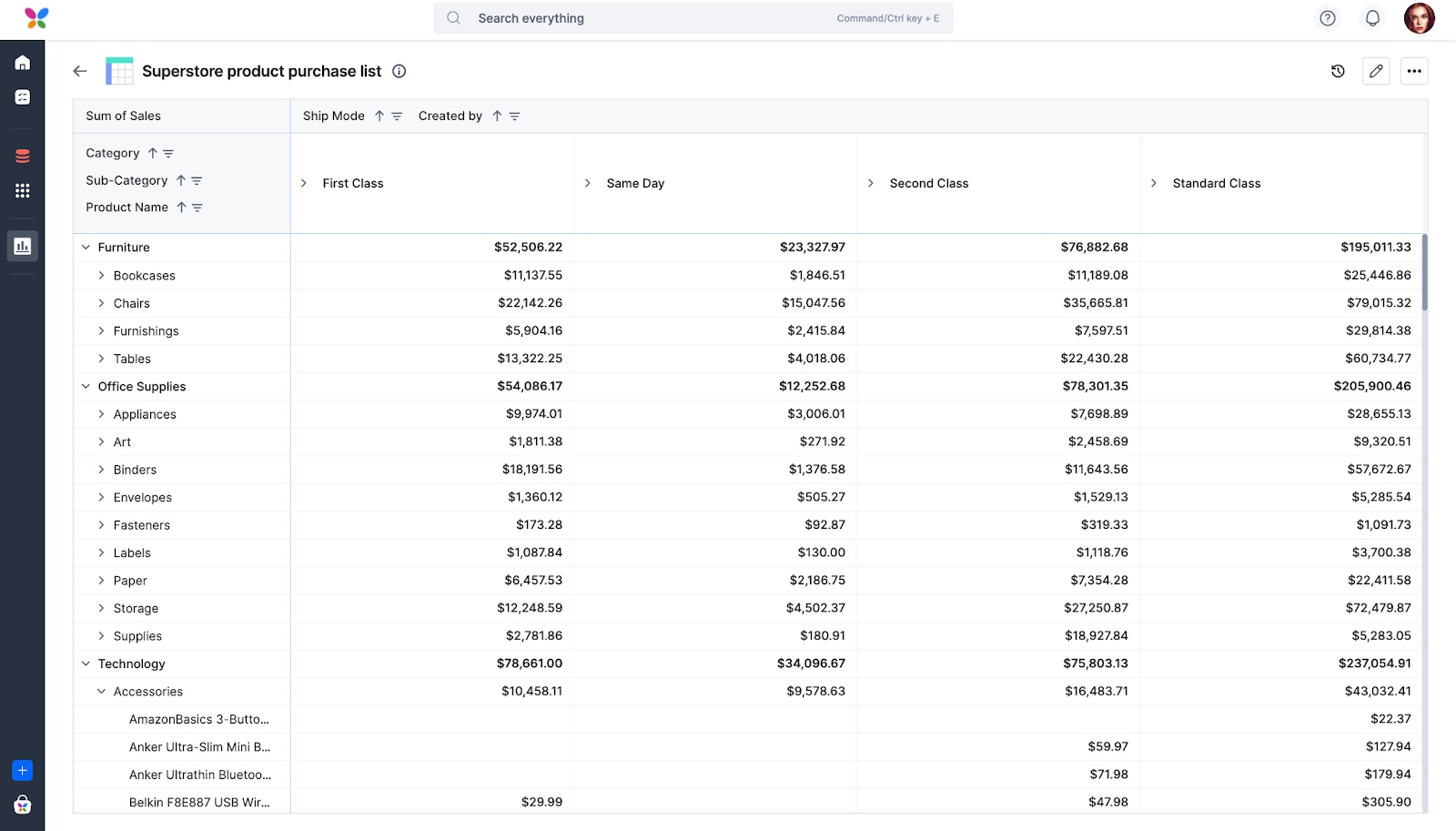
Pivot reports enable you to summarize, arrange, and compare a large amount of data effectively.
Creating a pivot report
Click the + Create report button on the Analytics page.
Select the data source.
Provide a name.
Select the type of report - Pivot.
Click Create.

Settings
Under settings, you can select the fields based on columns, values and rows. There are two types of fields to choose from.
- Custom fields - These are fields you created on your process, board or dataset and are unique to your process, board or dataset.
- System fields - These are system-generated fields that are created by default for a process such as Name, Created by, Modified by, Created at, Modified at and Flow name.
Selecting fields
In the field selection, you can do the following:
Click + Add fields to add the required fields from the data source.
To remove a field, click the Delete button (
).
Click the drag-and-drop icon (
) to drag and drop columns, values, and rows.

Columns
Add fields as columns from the data source. The order of your selection creates the column hierarchy. You can rearrange column order using drag-and-drop for flexibility.
You can include up to 10 fields as columns, and subtotal columns are automatically generated for consecutive levels, with Total appended to the column name.
Values
Under Values, select a field for aggregated values. Choose from aggregation types such as Sum, Average, Count, Min, Max, or Variance. You can only add one field.
Rows
Add fields as rows from the data source. The selection order defines the row hierarchy. Successive rows follow the initial row based on field order.
You can add up to 10 fields as rows. Use drag-and-drop to place rows in your preferred order.
Tip: If you hover over a cell value, you can see which row and column it belongs to, along with the value.
Filtering data
To narrow down specific data in your pivot table, you can add filters. Click Advanced filter to add a filter to your report during configuration. Choose the fields you want to filter and enter the conditions. Click Save to configure the report.
Click + Add new filter button to add more filters and conditions to the same field. The new condition can be either AND (all conditions must be met) or OR (any one condition must be met). Learn more about how to use advanced filters.

Grand totals
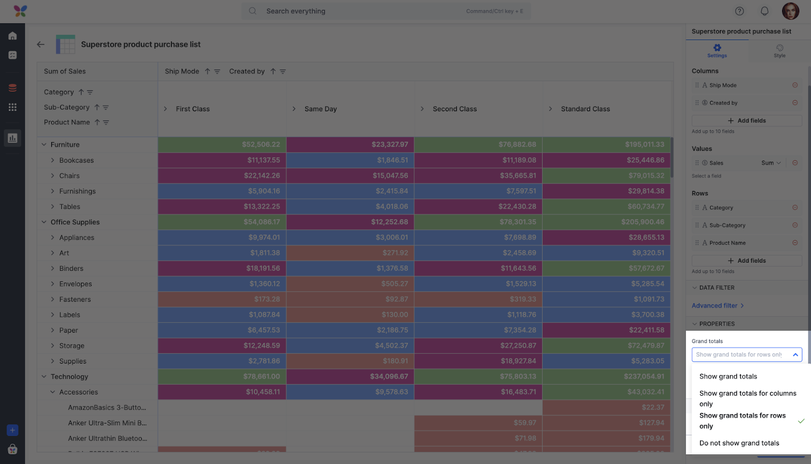
Under Grand totals, select how you want to display grand totals.
Show grand totals - display grand totals for all rows and columns.
Show grand totals for columns only - display grand totals for each column.
Show grand totals for rows only - display grand totals for each row.
Do not show grand totals - hide grand totals for all rows and columns.
Value calculations
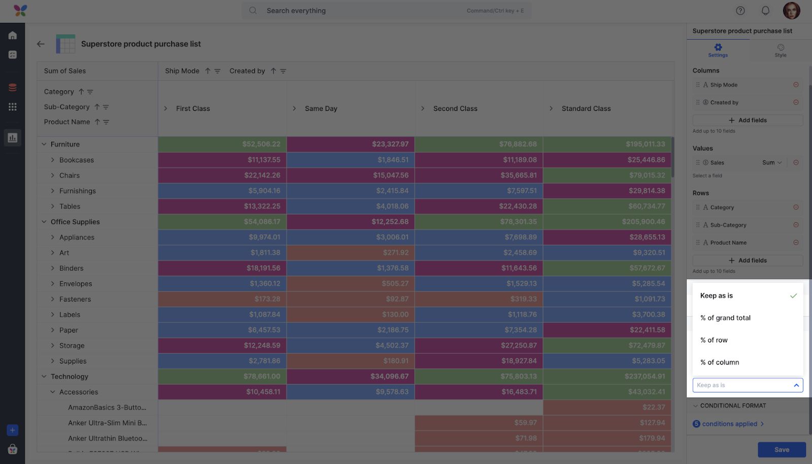
Under Value calculations, select how you want to calculate values.
Keep as is - the values don’t change.
% of grand total - the table values will be displayed in percentage instead of sum.
% of row - the row total will be shown in percentage instead of sum.
% of columns - the column total will be displayed in percentage instead of sum.
Conditional formatting
Conditional formatting enables you to visually enhance data cells within a pivot table using various styles, depending on specified conditions. This functionality allows you to color code and categorize data for simplified analysis.
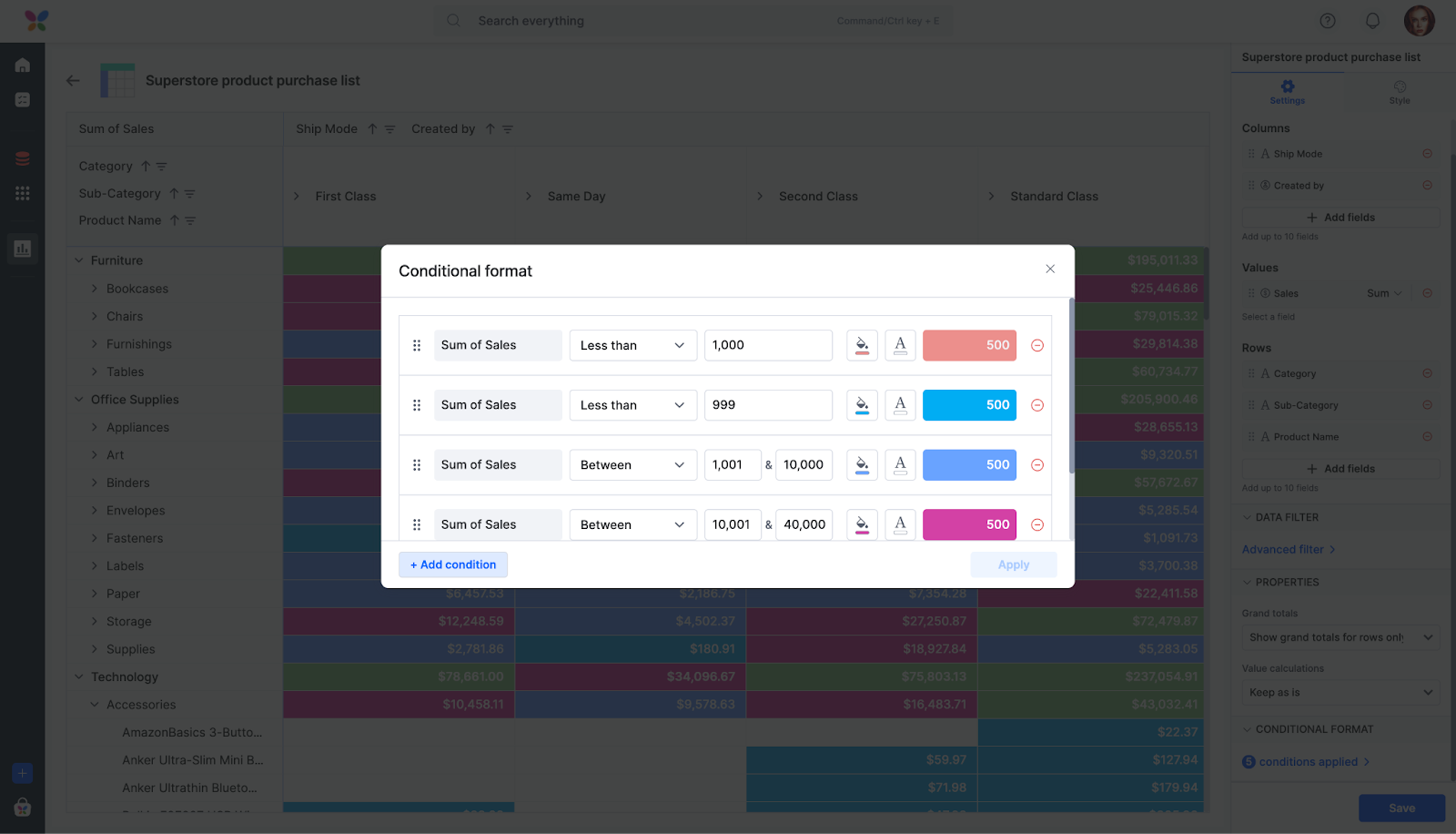
During report configuration, you can customize the appearance of your data cells, including value and background color, by defining conditions. These conditions can be based on cell values, such as equal to, not equal to, greater than, less than, greater than or equal to, less than or equal to, between, and not between.
Follow these steps to apply conditional formatting.
Under Conditional format, click Add condition > + Add condition.
Select the condition you want to apply to the cell.
Enter the value.
Format the cell’s background color and font color.
Click Apply.

You can easily rearrange conditions by using drag-and-drop during the addition process. In case of two conditions with the same value range, the latest condition applied through drag-and-drop will take precedence. You can then edit them based on your requirements.
You can add any number of conditions. The specified conditions are evaluated from top to bottom, and the formatting options associated with the first matching condition are applied to the respective data cell. To remove a condition, click Remove condition icon ().
Note:
Conditional formatting will not be applied for column and row totals (column based totals and row based totals) and grand totals.
Applying styles to pivot reports
Format the column header, cells, and grand totals of your report to suit your preferences. Choose the Normal state for the default appearance and the Hover state to preview styles on hovering.
Header section: Customize the background color, font size, font color, font weight, and icon color of the column header. The font weight dropdown provides options like Regular, Medium, and Semi-bold.
Cell settings: Adjust the Font size, Font color, Font weight, Line height, and Letter spacing for the cells in your pivot report.
Grand total customization: In the grand total section, you can adjust the background color, Font color, and Font weight of the grand total section of your report.

Additional actions
Once you have configured and saved your report, you can perform actions such as rearranging rows and columns, applying filters, customising the view by expanding/collapsing pivot levels, and formating currency fields.
Sort: Arrange your rows and columns in ascending or descending order using the Sort button (
). Rows and columns are sorted in ascending order by default.
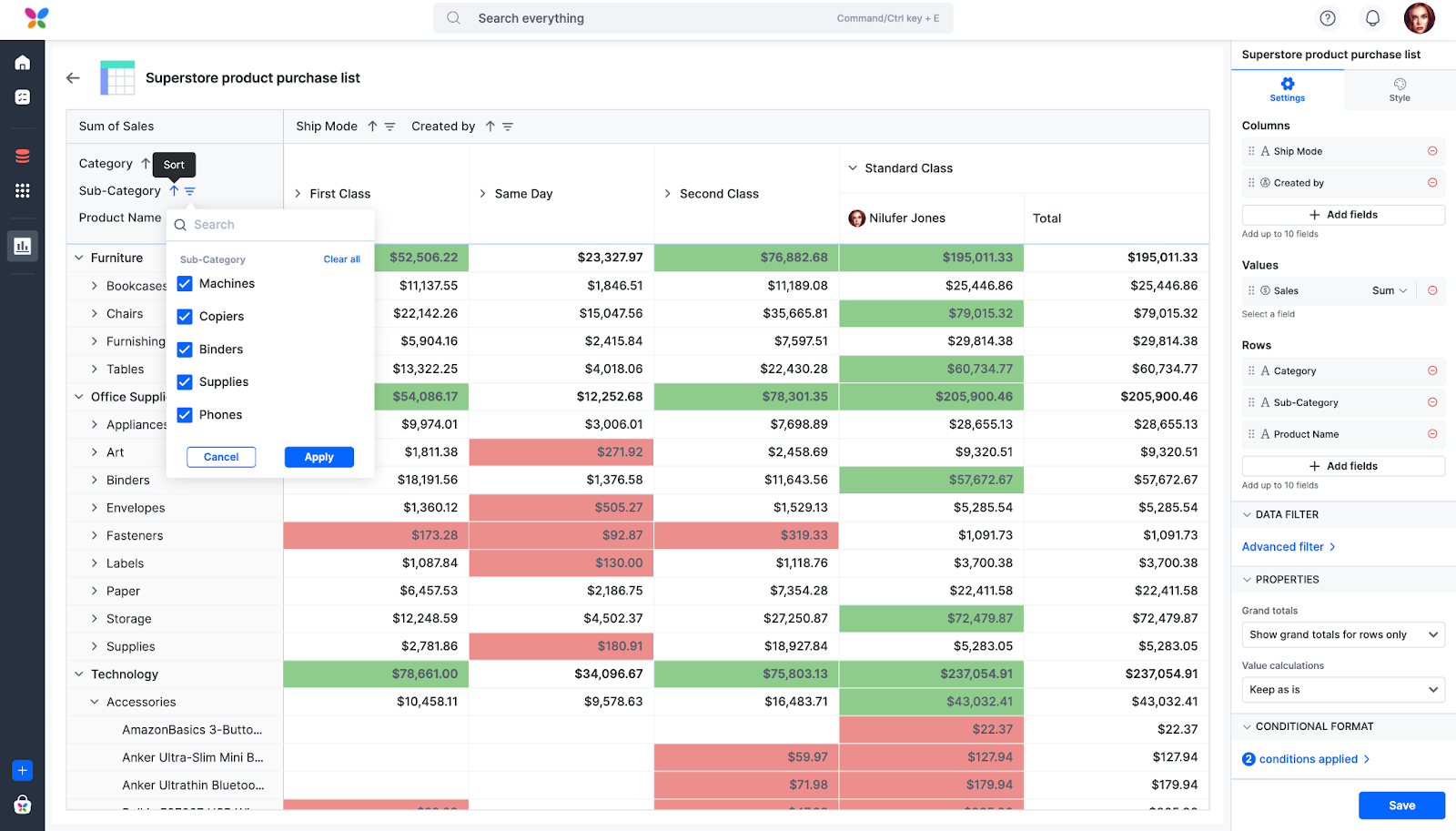
Filter: To filter by specific rows or columns, click the Filter icon (
) beside the row/column > use search box to easily identify the fields or select the checkboxes next to the items you want to show > click Apply. Use Select all and Clear all to easily filter the items.
Expand/collapse: Click Expand to see details of a section or Collapse to hide them. The chosen state (expand/collapse) is saved even if you leave the page.
Widgets: When selecting a currency-type field in Values, the currency format will be applied to the fields. User fields in rows and columns will be presented in a user widget format similar to forms.
Note:
If a currency field value has various currency type formats, they will be displayed as numbers without any currency formatting.
Use case
If you want to create a purchase catalog report in which you can compare the totals for each row, then pivot report is the right choice. The report gives you a quick overview of the data by displaying grand totals depending on the specific needs of the user.
For instance, a sales manager can use a pivot report to analyze sales data by product category, customer, or sales representative. The manager can use the grand totals to see the total number of customers in each age group, location, or product purchased.